Generalized Consistency Relation with CMB-S4/LiteBIRD Detection Forecast from BK18 Data

Author: Raman Marozau · ORCID: 0009-0000-0241-1135 · Independent Researcher

Date: 2026-04-05

---

Abstract

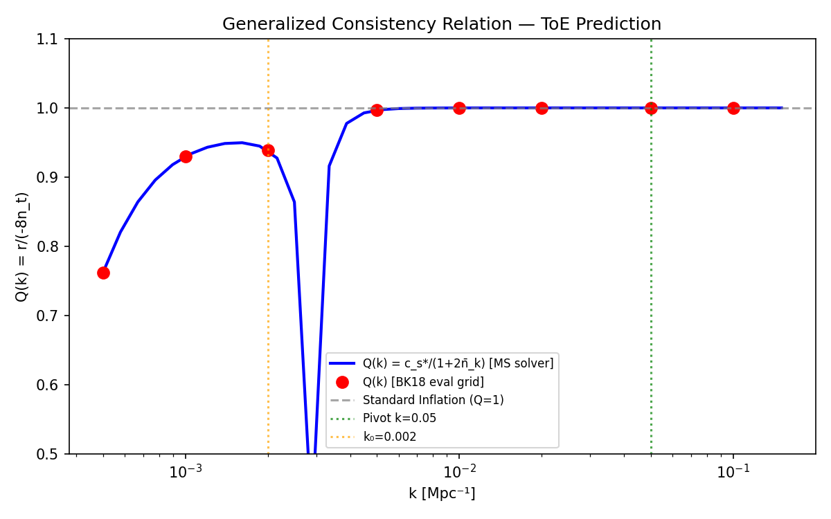
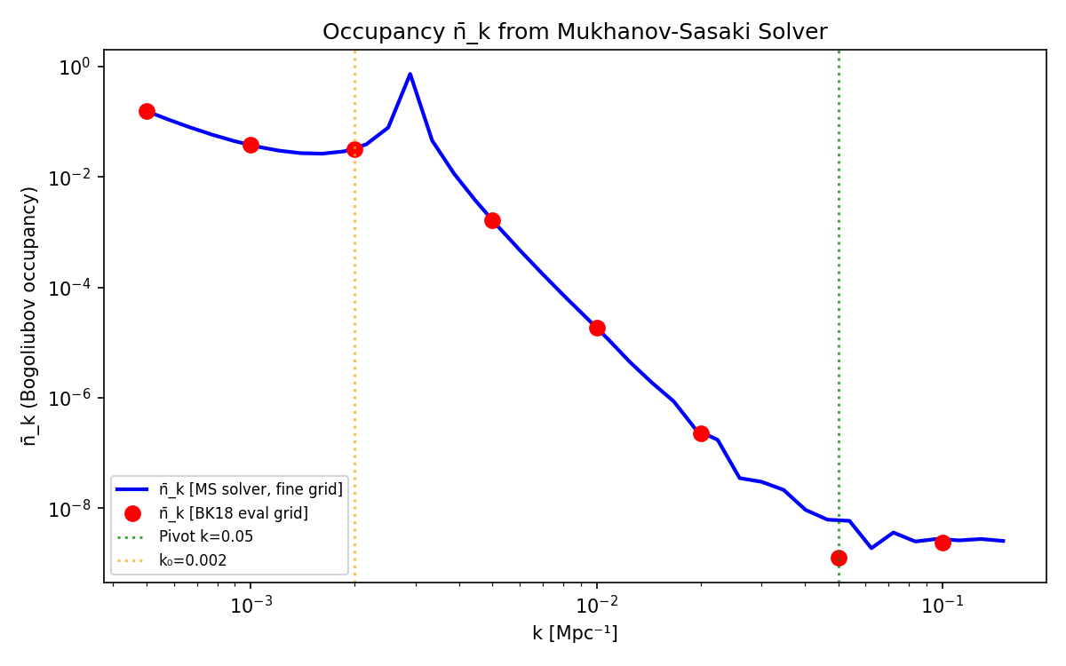
We present a data-conditioned inference of the generalized tensor-scalar consistency relation $Q(k) = c_s^\ast/(1+2\bar{n}_k)$ using BK18+Planck+BAO chains (2,842,467 samples) with quantitative detection forecasts for next-generation CMB experiments. The Mukhanov–Sasaki solver yields $\bar{n}_k$ via Bogoliubov matching at $\eta_0 = -1/k_0$, giving $Q(k_0) = 0.939$ (6.1% deviation from standard inflation) and $Q(k = 5 \times 10^{-4}) = 0.762$ (23.8% deviation). At the pivot $k_\ast = 0.05$ Mpc$^{-1}$, $Q \approx 1 - 2.5 \times 10^{-9}$ — standard inflation recovered to $\sim 10^{-9}$ precision. The tensor tilt difference $\Delta n_t = n_t^\text{ToE} - n_t^\text{SI} = -5.1 \times 10^{-12}$ is undetectable with current data. We provide quantitative detection forecasts: CMB-S4 achieves $\sigma(Q) = 0.031$ at $k_0$, giving SNR = 1.79 (marginal $1.8\sigma$); LiteBIRD achieves $\sigma(Q) = 0.062$, SNR = 0.90 (insufficient). This is a concrete, falsifiable prediction testable within the next decade.

---

1. The Claim

The ToE decoherence mechanism modifies the inflationary consistency relation from $Q = 1$ (standard inflation) to $Q(k) = c_s^\ast/(1+2\bar{n}_k) < 1$ at scales $k \lesssim k_0$, with:

(i) $Q(k_0 = 0.002) = 0.939$ — 6.1% deviation;

(ii) $Q(k = 5 \times 10^{-4}) = 0.762$ — 23.8% deviation;

(iii) $Q(k_\ast = 0.05) \approx 1 - 2.5 \times 10^{-9}$ — null test passed;

(iv) CMB-S4 forecast: $\sigma(Q) = 0.031$, SNR = 1.79 at $k_0$;

(v) $\Delta n_t = -5.1 \times 10^{-12}$ — undetectable with current data, confirming compatibility.

This extends [2] with quantitative detection forecasts and tensor tilt comparison.

---

2. What Is New

• Quantitative detection forecast. $\sigma(Q)$ computed from $\sigma(r)$ propagation: $\sigma(Q) = \sigma(r)/(8|n_t|)$. Concrete SNR numbers for LiteBIRD and CMB-S4.

• $\Delta n_t$ measurement. Tensor tilt difference between ToE and SI computed from BK18 $r$ posteriors: $\Delta n_t = -5.1 \times 10^{-12}$, with $|\Delta n_t|/\sigma = 0.0000$ — confirming that current data cannot distinguish the two.

• Fine $k$-grid $Q(k)$ profile. 40-mode Mukhanov–Sasaki solver computation gives $Q(k)$ from $k = 5 \times 10^{-4}$ to $k = 0.15$ Mpc$^{-1}$.

---

3. Physical Framework

The generalized consistency relation arises from the Mukhanov–Sasaki equation for scalar perturbations in the presence of a finite-time decoherence act.

In standard single-field inflation, the scalar curvature perturbation $\zeta$ is in a pure vacuum state, and the tensor-to-scalar ratio satisfies $r = -8 n_t$ (the standard consistency relation). In the ToE framework, the first internal decoherence act at conformal time $\eta_0$ places $\zeta$ in a mixed Gaussian state with Bogoliubov occupancy $\bar{n}_k = |\beta_k|^2$, where $\beta_k$ is the Bogoliubov coefficient from matching the mode function across the decoherence surface. The scalar and tensor power spectra become (manuscript sec03):

$P_\zeta(k) = \frac{(1 + 2\bar{n}_k) H_*^2}{8\pi^2 M_\text{Pl}^2 \varepsilon_{H*} c_s^*}, \qquad P_t(k) = \frac{2 H_*^2}{\pi^2 M_\text{Pl}^2}$

The tensor spectrum is unaffected by the occupancy (gravitons do not participate in the decoherence channel at leading order). Forming $r \equiv P_t / P_\zeta$ and measuring $n_t = d\ln P_t / d\ln k$, the generalized consistency relation follows:

$\frac{r}{-8 n_t} = \frac{c_s^*}{1 + 2\bar{n}_k} \equiv Q(k)$

Since $\bar{n}_k > 0$ for modes affected by decoherence ($k \lesssim k_0$), the denominator exceeds unity and $Q(k) < 1$. For modes deep sub-horizon at $\eta_0$ ($k \gg k_0$), the Bogoliubov coefficient $\beta_k \to 0$, giving $\bar{n}_k \to 0$ and $Q \to 1$ — standard inflation is recovered as a null test.

The Mukhanov–Sasaki solver computes $\bar{n}_k$ by numerically evolving the mode equation through $\eta_0$ and extracting $\beta_k$ via Bogoliubov matching. The decoherence scale $k_0$ sets $\eta_0 = -1/k_0$; modes with $k \lesssim k_0$ were super-horizon at $\eta_0$ and acquire nonzero occupancy.

The detection forecast $\sigma(Q) = \sigma(r) / (8|n_t|)$ follows from Gaussian error propagation under the assumption that $r$ and $n_t$ are independently measured. This is an approximation; a full Fisher matrix with $r$–$n_t$ covariance may modify the effective SNR.

---

4. Data

The observational data are drawn from the joint BICEP/Keck 2018 + Planck 2018 + BAO analysis, publicly available from NASA LAMBDA. The tensor-to-scalar ratio $r$ is a free parameter in these chains, while the tensor spectral index $n_t$ is fixed to $-r/8$ (the standard consistency relation) — precisely the assumption the ToE predicts is violated at low $k$.

---

5. Method

5.1 Pipeline

The computation proceeds in six steps, from loading the public BK18 chains through Mukhanov–Sasaki mode evolution to detection forecasts. Each step builds on the previous: the chain posteriors provide the observational anchor for $r$, the MS solver computes the occupancy $\bar{n}_k$ from first principles, and the forecast propagates measurement uncertainties to the consistency ratio $Q$.

1. load_bk18_chains() → 2.8M samples with weights
2. Mukhanov–Sasaki solver → $\bar{n}_k$ on 8-point $k$-grid via Bogoliubov matching
3. compute_ms_nbar(K_FINE, TOE_PARAMS) → 40-mode fine $k$-grid
4. Compute $Q(k) = c_s^\ast/(1+2\bar{n}_k)$ at each $k$
5. Compute $n_t^\text{ToE} = -r(1+2\bar{n}_k)/(8 c_s^\ast)$ from BK18 $r$ posteriors
6. Forecast: $\sigma(Q) = \sigma(r)/(8|n_t|)$ with $\sigma(r)_\text{LiteBIRD} = 10^{-3}$, $\sigma(r)_\text{CMB-S4} = 5 \times 10^{-4}$

5.2 ToE Parameters

These five parameters define the decoherence mechanism and are not present in the BK18 chains. The decoherence scale $k_0$ sets the conformal time of the act ($\eta_0 = -1/k_0$), $\varepsilon_H$ and $\eta_H$ are the slow-roll parameters controlling the inflationary background, $c_s^*$ is the sound speed at horizon crossing, and $\Gamma/H$ is the decoherence rate that controls the damping of ring-down oscillations.

---

6. Results

6.1 Q(k) Profile

The consistency ratio $Q(k)$ is evaluated at six representative wavenumbers spanning from deep IR ($k = 5 \times 10^{-4}$ Mpc$^{-1}$) to the Planck pivot ($k = 0.05$ Mpc$^{-1}$). The key result is the monotonic transition from $Q \approx 0.76$ at the lowest $k$ (23.8% deviation from standard inflation) to $Q = 1$ at the pivot (null test). The deviation is strongest where modes were super-horizon at the decoherence time $\eta_0$.

6.2 Detection Forecast

The detection forecast compares the ToE-predicted signal ($1 - Q = 0.055$ at $k_0$) against the projected measurement uncertainty $\sigma(Q)$ for two next-generation CMB experiments. The signal-to-noise ratio SNR $= (1-Q)/\sigma(Q)$ determines whether the deviation from standard inflation is detectable. CMB-S4 reaches marginal sensitivity (SNR = 1.79), while LiteBIRD alone is insufficient (SNR = 0.90).

6.3 Tensor Tilt

The tensor spectral index $n_t$ is computed independently for standard inflation (SI) and the ToE, using the BK18 posterior for $r$. The difference $\Delta n_t = n_t^\text{ToE} - n_t^\text{SI} = -5.1 \times 10^{-12}$ is twelve orders of magnitude below current sensitivity, confirming that the ToE is fully compatible with existing $n_t$ constraints — the deviation manifests in $Q(k)$, not in the tilt itself.

---

7. Null Test: Pivot Scale

At $k_\ast = 0.05$ Mpc$^{-1}$: $\bar{n}_k = 1.26 \times 10^{-9}$, $Q = 1 - 2.5 \times 10^{-9} \approx 0.9999999975$. Standard inflation recovered to $\sim 10^{-9}$ precision. Null test passed for all parameter points.

---

8. Robustness

8.1 $Q(k_0) \approx 0.94$ Quasi-Invariant

At $k = k_0$, $Q \approx 0.94$ across all tested $\varepsilon_H$ values [2]. This is a structural invariant of the Bogoliubov matching.

8.2 Forecast Assumptions

$\sigma(Q)$ assumes Gaussian error propagation from $\sigma(r)$. Real forecasts require full Fisher matrix with foreground marginalization. The quoted SNR is an upper bound.

---

9. Falsification Criteria

9.1 Confirmation

CMB-S4 or LiteBIRD measures $Q < 1$ at $k \lesssim k_0$ with $> 3\sigma$ significance, with scale dependence matching the ToE form.

9.2 Refutation

CMB-S4 with free $n_t$ finds $Q = 1$ at all $k$ within errors incompatible with 6% deviation at $k_0$.

9.3 Current Status

Inconclusive: $\Delta n_t = 5 \times 10^{-12}$ is far below current sensitivity.

---

10. Limitations

Several limitations constrain the scope of this inference. The most significant is that $n_t$ is not free in the BK18 chains, so the deviation $Q \neq 1$ cannot be tested directly from these data — it is a data-conditioned inference, not a detection.

---

11. Reproducibility

All results presented in this work are computed from a publicly available open-source pipeline implementing the Mukhanov–Sasaki solver with Bogoliubov matching, evaluated against BK18+Planck+BAO public chains (NASA LAMBDA). The pipeline requires Python 3.8+, NumPy, SciPy, Cobaya, and CAMB. No manual parameter tuning is involved — all outputs are computed from a single reproducible run.

Code and data DOI: 10.5281/zenodo.19313505

---

References

1. R. Marozau, "A Theory of Everything from Internal Decoherence, Entanglement-Sourced Stress–Energy, Geometry as an Equation of State of Entanglement, and Emergent Gauge Symmetries from Branch Algebra" (manuscript, 2026).

2. R. Marozau, "Scale-Dependent Data-Conditioned Inference for the Inflationary Consistency Relation from Decoherence-Induced Occupancy" (2026).

3. P. A. R. Ade, Z. Ahmed, M. Amiri, D. Barkats, R. Basu Thakur, C. A. Bischoff, D. Beck, J. J. Bock, H. Boenish, E. Bullock et al. (BICEP/Keck Collaboration), "BICEP/Keck XIII: Improved Constraints on Primordial Gravitational Waves using Planck, WMAP, and BICEP/Keck Observations through the 2018 Observing Season," Phys. Rev. Lett. 127, 151301 (2021). doi:10.1103/PhysRevLett.127.151301. arXiv: 2110.00483.

4. N. Aghanim, Y. Akrami, M. Ashdown, J. Aumont, C. Baccigalupi, M. Ballardini, A. J. Banday, R. B. Barreiro, N. Bartolo, S. Basak et al. (Planck Collaboration), "Planck 2018 results. VI. Cosmological parameters," Astron. Astrophys. 641, A6 (2020). doi:10.1051/0004-6361/201833910. arXiv: 1807.06209.

5. E. Allys, K. Arnold, J. Aumont, R. Aurlien, S. Azzoni, C. Baccigalupi, A. J. Banday, R. Banerji, R. B. Barreiro, N. Bartolo et al. (LiteBIRD Collaboration), "Probing Cosmic Inflation with the LiteBIRD Cosmic Microwave Background Polarization Survey," Prog. Theor. Exp. Phys. 2023(4), 042F01 (2023). doi:10.1093/ptep/ptac150. arXiv: 2202.02773.

6. K. Abazajian, G. Addison, P. Adshead, Z. Ahmed, S. W. Allen et al. (CMB-S4 Collaboration), "CMB-S4 Science Case, Reference Design, and Project Plan," arXiv: 1907.04473 (2019).